
Suppose a decoder is working on the word bank. By the time its hidden vector reaches a mixture-of-experts layer, the surrounding words have already influenced that vector. In "the river flooded the bank," it can look different from the vector for the same token in "the bank raised rates." The router takes that contextual vector, scores the available experts, and picks a few to run. Their outputs are added back into the decoder's hidden stream.
That is the part I wanted to see clearly while working on C-Kernel-Engine (CKE). What does the router actually multiply? Where do the expert IDs go? And why does this part of the model use GEMMs that behave so differently from the GEMM at the language-model head?
1. Where MoE fits in the decoder
A decoder starts by turning token IDs into vectors of width H. Each layer reads and updates those vectors. Its token-mixing sublayer lets information travel between positions, using attention in a typical transformer or a mix of attention and recurrent layers in Qwen3.5. Its feed-forward sublayer transforms each position's features. A mixture of experts, or MoE, replaces that feed-forward sublayer with a bank of smaller feed-forward networks and a router.
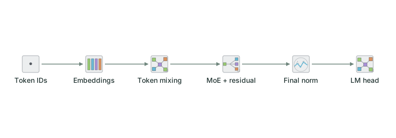
For the pre-normalized block in the diagram, call the post-mixing residual stream r. The feed-forward norm computes x = norm(r). The router reads x, the selected experts also read x, and the block returns r + mixture(x). Its output is still one H-wide vector per token. The next decoder layer can therefore use it just like the output of a dense feed-forward block. The language-model head sits after the decoder stack, usually after a final normalization.
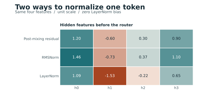
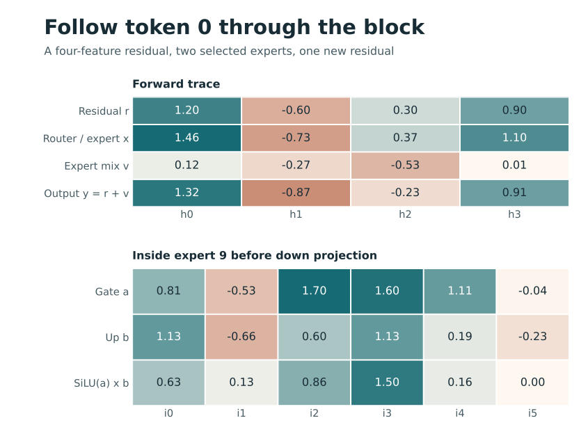
For example, four token IDs index four rows of an embedding table W_embed[V,4], giving an initial [4,4] hidden stream. Attention and earlier residual updates change the values while keeping that shape. The plots below start after token mixing, with a deliberately small residual row [1.2, -0.6, 0.3, 0.9] for token 0. That lets us see what the MoE changes without attributing the toy values to a real embedding or attention model.
What does FFN norm mean?
FFN means feed-forward network. FFN norm tells you where the normalization sits, in this case before the feed-forward branch. The model architecture tells you which normalization to use. The CKE Qwen3.5-MoE circuit uses RMSNorm at the step named post_attention_norm. It reads the stream after the first residual add and sends the same normalized row to the router, routed experts, and shared expert. The unnormalized row stays on the skip path to the second residual add. In the circuit, this puts the norm after token mixing and before the FFN.
RMSNorm:   x = gamma * r / sqrt(mean(r*r) + eps)

LayerNorm: u = r - mean(r)
           x = gamma * u / sqrt(mean(u*u) + eps) + beta
Both reduce over the H hidden features of one token, not across the sequence. RMSNorm divides by the root mean square without subtracting the mean. LayerNorm first centers the row, then uses the variance of that centered row; its affine form can learn both a scale and an offset. The two can produce different router scores even with identical router weights. For example, adding the same constant to every feature leaves LayerNorm unchanged with fixed parameters, whereas RMSNorm generally changes.
2. What a router actually looks like
Start with T hidden rows, each of width H. If the layer has E routed experts, give the router one weight row per expert. In output-row-first notation the matrix is W_router[E,H]. A dot product with row e gives expert e's score for a token. One dense matrix multiplication computes all those scores:
X         [T,H]   normalized hidden features
W_router  [E,H]   learned router weights
S         [T,E]   X times transpose(W_router)

ids       [T,K]   selected expert IDs
weights   [T,K]   corresponding mixture weights
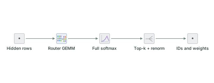
The projection produces S. The routing policy reads S and produces ids and weights. That separation is visible in CKE's Qwen3.5 circuit spec: gemm_nt_f32_llama_production is the score projection, and moe_softmax_topk_router_llama_f32 is the selected softmax/top-k kernel family. The workspace entry point in topk_kernels.c accepts logits and writes IDs and weights. Its scratch buffer holds a probability row that it reuses across input rows.
What happens in top-k + renorm?
Top-k answers "which experts run?" Renorm answers "how much of each result do we use?" Take four experts and keep two. One token gets logits [2, 1, 0, -1]. Full softmax divides across all four scores. Top-k then keeps the IDs of the two largest probabilities. Renorm divides those two probabilities by their own sum, not by the number of experts.
| Expert | Logit | Full softmax | After renorm |
|---|---|---|---|
| 0 | 2 | 0.644 | 0.731 |
| 1 | 1 | 0.237 | 0.269 |
| 2 | 0 | 0.087 | Not run |
| 3 | -1 | 0.032 | Not run |
ids          = [0, 1]
kept         = [0.644, 0.237]
kept mass    = 0.644 + 0.237 = 0.881
weights      = [0.644 / 0.881, 0.237 / 0.881]
             = [0.731, 0.269] approximately
expert mix   = 0.731 * expert_0(x) + 0.269 * expert_1(x)
The ratio between the two winners stays the same. What changes is their total: without renorm they carry about 88% of the original probability mass; with renorm they carry the whole mixture, before any model-specific scale. There is no dense vector of expert outputs to multiply by zeros. The runtime keeps two pairs, (expert ID, weight), and dispatches only those two experts for this token. Open the Top-k + renorm inspector to see where those pairs come out of the router.
In CKE, topk_f32 keeps a list of K candidates. As it scans the remaining scores, a better score replaces the weakest candidate. It sorts the final list of K, rather than sorting all E scores. If scores tie at the cutoff, a different tie policy can keep a different expert, so matching a reference implementation takes more than matching the formula.
CKE's softmax path subtracts the row maximum before exponentiating, then applies full softmax, selects top-k, and renormalizes the selected entries with a denominator floor and the model's routing scale. That is one policy. CKE also documents a group-limited sigmoid router where a correction bias can affect which experts get picked, while the selected weights come from the underlying sigmoid scores. Swapping the policy can change the expert IDs even if the router matrix is the same.
Ten experts, one decision GEMM
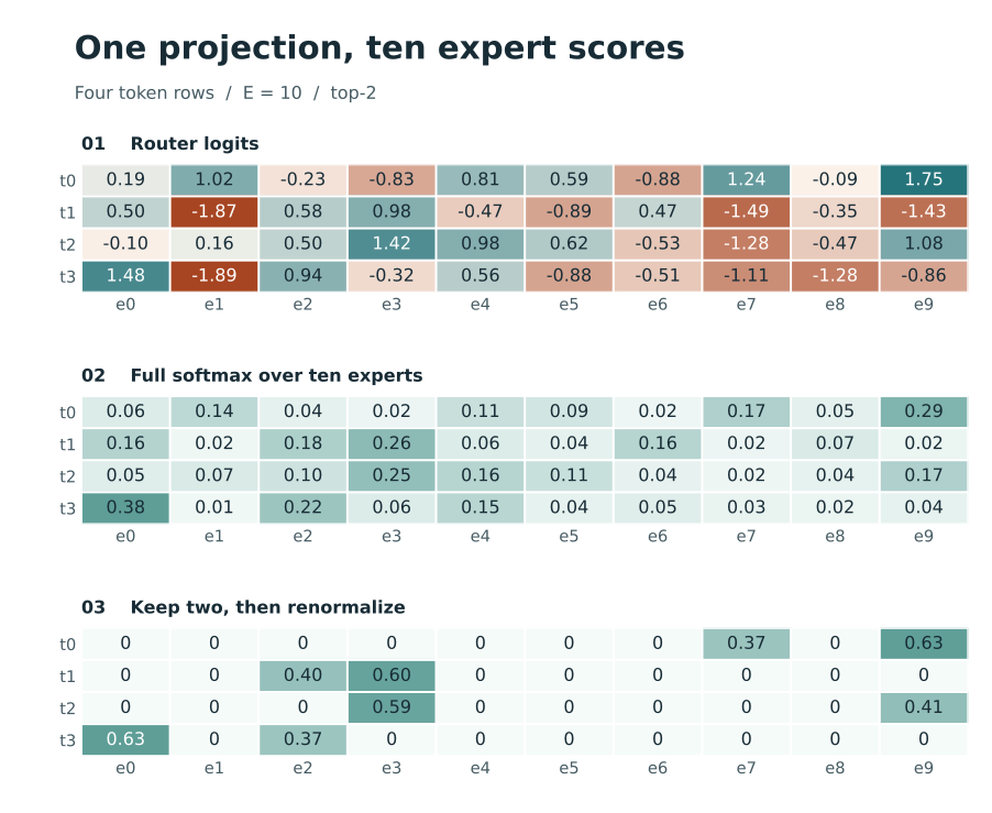
Let's build a small block with four token rows, hidden width four, ten experts, and expert intermediate width six. Imagine each expert were just a linear transformation. You would store ten expert matrices and one router matrix. In the SwiGLU version we actually use, each of those ten experts owns three projections: gate, up and down. The router is still one projection.
T = 4 tokens    H = 4 features    E = 10 experts    I = 6    K = 2

X [4,4] @ transpose(W_router [10,4])  -> logits [4,10]
top-k per row                         -> ids [4,2], weights [4,2]

Expert e receives X_e [n_e,4]:
  X_e @ transpose(W_gate[e] [6,4])    -> gate [n_e,6]
  X_e @ transpose(W_up[e]   [6,4])    -> up   [n_e,6]
  SiLU(gate) * up                     -> mid  [n_e,6]
  mid @ transpose(W_down[e] [4,6])    -> out  [n_e,4]
There is no rule that the router needs the same number of input and output features. Its input width is the width of the hidden state; its output width is the expert count. A square [10,10] router works when the incoming vector also has ten features. If the model has H = 4 and E = 10, it needs a rectangular [10,4] projection. Counting the same way for the whole block, there are 30 expert weight matrices plus the router, but each top-2 token uses only six expert matrices. A runtime can batch or fuse those multiplies, so that count is not a count of kernel launches.
Could the router just take the maximum?
Yes. If all you want is the index of the winning expert, scan the logits and take argmax. For finite, distinct scores, softmax preserves their order: exponentiation is increasing and every entry is divided by the same positive sum. Top-k can therefore use the raw logits as well, in exact arithmetic. Ties and finite-precision behavior still matter when reproducing a particular kernel.
For selection alone, softmax adds work. Argmax scans E scores. Full softmax also exponentiates those scores, sums the exponentials, and normalizes the row. The expert computation can be far more expensive than either choice, so the cost of the entire block still depends on the hardware and the shapes.
- Hard top-1: run the winner with weight 1. This is a valid inference policy, and a simple baseline if the router was trained for it.
- Normalize the top-k: run the selected experts and blend their outputs. The score gaps determine the weights. Selection alone cannot tell you whether the first two experts should contribute 51/49 or 99/1.
- Keep full-softmax weights for the winners: run only the selected experts but retain their original probabilities. Their weights need not sum to one. With top-1, the winning score still controls the amplitude and can carry a task gradient back to the router. Switch Transformer is an example of probability-scaled top-1 routing.
There is a useful simplification when the rule is normalize the selected weights. Let S be the selected IDs, p_i the full-softmax probability, and z_i the raw logit. The common full-softmax denominator cancels:
alpha_i = p_i / sum(p_j for j in S)
        = exp(z_i) / sum(exp(z_j) for j in S),  i in S
So you can select on raw logits and apply a stable softmax to just the winners, evaluating K exponentials rather than E. This is the same mixture in exact arithmetic if there is no active denominator floor, with the same routing scale applied afterward. It is not a guarantee of bitwise parity, and it cannot replace full softmax if another part of your training recipe uses the whole probability row. CKE's llama-compatible workspace follows its own full-softmax contract for that reason: the operation order, tie handling, and numerical guardrails are part of what gets compared to the reference.
3. What an expert computes
Each routed expert owns its own feed-forward weights. In a SwiGLU expert, the gate and up projections both take the original normalized row x and expand it to width I. Apply SiLU to the gate and multiply it element by element with the up projection. Then project down to H:
gate_e = W_gate[e]  x    // [I,H] times [H] gives [I]
up_e   = W_up[e]    x    // [I,H] times [H] gives [I]
mid_e  = SiLU(gate_e) * up_e
out_e  = W_down[e]  mid_e // [H,I] times [I] gives [H]

mixture(x) = sum over selected e: weight_e * out_e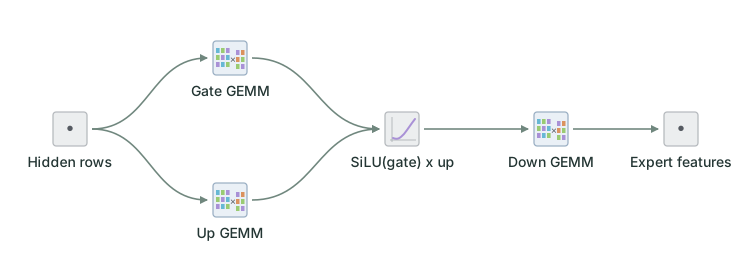
n_e counts the rows assigned to that expert.The two uses of gate can get confusing. The router gives the entire expert a scalar weight for this token. The SwiGLU gate lives inside that expert and has I entries, one for each intermediate feature. The expert's internal gate shapes its output; the router's weight scales that finished output.
To finish the toy example, say expert 0 returns [2, 0, 1] and expert 1 returns [0, 4, 3]. The weighted result is approximately [1.462, 1.076, 1.538]. The block adds that vector back to r. Some architectures also have a shared expert that runs for every token. The Qwen3.5-MoE path described in the CKE docs adds a shared expert behind its own learned sigmoid gate; that path is separate from the top-k expert list.
4. Why an expert GEMM is a scheduling problem
The multiply inside one expert is ordinary matrix math. The complication is getting the right rows to the right matrices. A dense feed-forward layer applies the same weight matrix to all T rows. In an MoE layer, two adjacent tokens can pick different expert IDs, and the same token may appear in several experts' input batches. A runtime that loops over tokens and experts as it finds them can turn a big prompt into thousands of small calls with scattered weight reads.
In the grouped Qwen3.5-MoE prefill path, CKE uses the router's IDs to bucket rows by expert within each routing slot. Each resulting segment feeds a GEMM using that expert's weights. The runtime keeps track of each row's original token and mixture weight so the contributions can be accumulated in the right output row. That bookkeeping is the dispatch and combine around the GEMMs.
Take the CKE docs' example: 512 prompt tokens, 256 available routed experts, and top-8. There are 512 * 8 = 4,096 token-expert assignments. Grouping does not eliminate those assignments. It lets several rows reuse the same expert weights in one segment and lets the runtime quantize the input rows once instead of repeating that work for every assignment. A single-token decode step has far fewer rows to group, so expert weight access, quantized dot products, and call overhead become more visible. Decode with several concurrent sequences can give the scheduler more rows to work with again.
The concrete mixed-quant example in CKE uses Q4_K gate/up weights, Q5_K down weights, Q8_K activations on the routed path, and routing-weighted accumulation into FP32. Those types describe the storage and compute contract of that provider, rather than requirements of MoE itself. The circuit, kernel map, and router parity tests let us check those pieces separately. When an output diverges, I can compare router logits, selected IDs, weights, and finally the weighted expert output. Comparing the final vocabulary logits alone leaves a lot more code to search.
5. Router, expert, LM head, and classifier
| Operation | Typical shape | Who uses the result? |
|---|---|---|
| Router projection | [T,H] to [T,E] | Top-k routing turns expert scores into a work list and mixture weights. |
| Expert projections | [n_e,H] to [n_e,I] to [n_e,H] | The combine step returns new hidden features to the decoder. |
| Language-model head | [T,H] to [T,V] | Training loss or a sampler reads vocabulary logits. Decode often projects only the last row per sequence. |
| Linear classifier | [B,H] to [B,C] | A loss or application reads label logits, often after pooling each example to one feature row. |
Look at what each column means. In the router, column 7 can mean "expert 7 in this layer." In the LM head, column 7 is a tokenizer vocabulary ID. In a classifier, it could be the eighth application label. The router and the two linear heads can look very similar if you only inspect the matrix multiply. What follows the multiply tells you which one you're looking at. Router top-k dispatches hidden rows inside the model. Sampler top-k filters candidate tokens at the output. Classifier scores can go straight to an application decision.
A Clef decision head makes the contrast concrete. In CKE's registered supplied-feature recipe, a small supervised head learns from labeled backbone features while the backbone stays frozen. It predicts a task label, such as a support category. An MoE router learns an internal choice that helps the network's training objective. Expert IDs are not application labels, and there is no reason to name them "math" or "code" just because a few prompts happen to select them.
6. What the active parameter count buys you
Top-k routing lets the model store many expert weights without running all of them for every token. The Qwen3 technical report, for example, describes MoE models with 128 routed experts and 8 selected for each token. That ratio applies to the routed expert bank; attention, embeddings, the router, and the output projection still have their own costs. A batch may collectively touch many more than eight experts, and the full weight set still needs storage and a way to reach the compute device.
That is where the systems trade-off sits. During training, routing can concentrate work on a handful of experts, which is why sparse-model recipes often use some form of load balancing. During inference, skewed expert usage changes how well the grouped kernels fill up, and on a distributed system it can change how much traffic each device has to handle. The Switch Transformer paper is a useful introduction to those training and communication costs. For the CKE side, the place to pick up the thread is the grouped prefill trace: follow the IDs out of the router and see exactly what rows the GEMM receives.
7. Backpropagate through the MoE block
Use one token and column vectors for the derivation. Let y = r + v, x = RMSNorm(r), and v = sum_e alpha_e f_e(x) over the selected set S. Write d_u for dL/du, and call the upstream vector g = d_y. The derivation assumes a fixed selected set away from a top-k boundary, selected-softmax weights with scale 1, no bias, no shared expert, and an inactive normalization floor.
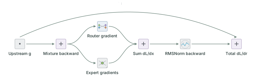
g unchanged.Start at the residual add and mixture
Both inputs of an addition receive the same upstream gradient. The direct skip contributes g to d_r. The mixture also receives g. Each scalar-vector product then splits that gradient again:
d_v          = g
d_r via skip = g
d_f_e        = alpha_e * g
d_alpha_e    = dot(g, f_e)
The scalar d_alpha_e is how much changing this expert's weight would change the loss locally. The vector d_f_e tells the expert how its features should move and scales that signal by its routing weight.
Differentiate one SwiGLU expert
Write a = W_gate x, b = W_up x, m = SiLU(a) * b, and f = W_down m. The symbol * is elementwise here. With s = sigmoid(a), SiLU(a) = a * s and SiLU'(a) = s + a * s * (1 - s). The down projection gives the first two lines, the product and SiLU give the middle two, and the two input projections give the rest:
d_W_down = outer(d_f, m)                // [H,I]
d_m      = transpose(W_down) @ d_f      // [I]
d_a      = d_m * b * (s + a*s*(1-s))    // [I]
d_b      = d_m * (a*s)                  // [I]
d_W_gate = outer(d_a, x)                // [I,H]
d_W_up   = outer(d_b, x)                // [I,H]
d_x_e    = transpose(W_gate) @ d_a
         + transpose(W_up)   @ d_b      // [H]
Add the parameter-gradient outer products over all token rows assigned to that expert. For a whole expert bucket those sums are matrix multiplies: for example, d_W_gate = transpose(D_a) @ X_e. Unselected experts have no task gradient from that token. CKE's FP32 expert backward kernel shows this split in C: it takes selected IDs and routing weights and returns gradients for expert weights, hidden input, and routing weights. The expert kernel does not differentiate the router itself.
Differentiate the router
With the selected IDs held fixed, the softmax Jacobian inside that set is d alpha_i / d z_j = alpha_i * (delta_ij - alpha_j), where delta_ij is 1 for the same index and 0 otherwise. Contract it with the weight gradients from the mixture:
mean_d_alpha = sum(alpha_i * d_alpha_i for i in S)
d_z_j        = alpha_j * (d_alpha_j - mean_d_alpha), j in S
d_z_j        = 0,                                 j outside S

d_W_router   = outer(d_z, x)       // [E,H]
d_x_router   = transpose(W_router) @ d_z
d_x          = d_x_router + sum(d_x_e for e in S)
The integer route itself has no ordinary gradient. At a boundary where one expert replaces another, the mixture can jump, so these are local derivatives on one side of that boundary. With selected normalization and K = 1, the sole weight is 1 and the task gradient through that weight is zero; the expert and the residual still train. With unrenormalized top-1, the selected weight is p_i from the full softmax, and d_z_j = d_p_i * p_i * (delta_ij - p_j). Now even unselected logits can get a gradient through the full-softmax denominator. Load-balancing losses can provide another router signal; the particular loss is a training choice, not something the top-k index operation differentiates.
Go back through RMSNorm and add the skip
For learned feature scales gamma and fixed eps, let s_r = sqrt(mean(r*r) + eps) and x = gamma * r / s_r. Changing any feature changes the common denominator, so the backward pass has a correction shared across the row:
q           = gamma * d_x
d_gamma     = d_x * r / s_r             // sum over token rows
d_r_branch  = q / s_r - r * mean(q*r) / s_r^3
d_r         = g + d_r_branch
If the block also has a shared branch sigmoid(w_s dot x) * f_s(x), that branch receives the same g at the sum. For beta = sigmoid(w_s dot x), its expert receives beta * g, and its gate-logit gradient is dot(g, f_s) * beta * (1-beta). Add both shared-branch input gradients into d_x before RMSNorm backward. The original residual skip still contributes g.
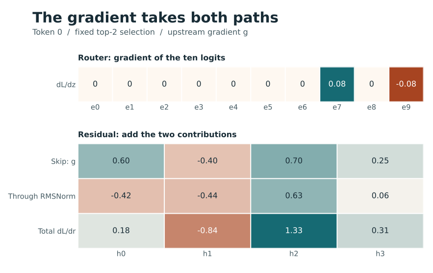
The plots use a reproducible NumPy example with a scalar loss L = sum(y * g). I checked every input feature, RMSNorm scale, router weight, and expert weight with central finite differences, keeping the selected IDs unchanged under the perturbations. The maximum absolute error was about 1.1e-10 in float64. That checks the equations for the toy block; it is separate from CKE's model and kernel parity tests.
8. Follow a routed token into CKE
If you want to trace this in code, start with the expert IDs for one token. The circuit decides which routing rule to use. The router returns IDs and mixing weights. The expert kernel uses those IDs to find the matrices it needs. That gives you three places to look when the final number seems wrong.
- Which rule did this model ask for? Read the Qwen3.5 circuit alongside the Nemotron-H circuit. Qwen’s softmax example and Nemotron’s group-limited selection answer the same question in different ways.
- Which experts won, and by how much? Follow the softmax router map into the C implementation. Read one row of logits and track the selected IDs separately from the floating-point weights. The router test gives you inputs and a reference result to compare.
- Where is the matrix work? Follow the Qwen grouped prefill path into the expert accumulation kernels. During prefill, many tokens can select the same expert. Gathering those rows lets the runtime reuse that expert’s weights before moving to the next one. The illustrated kernel guide traces the buckets, packed matrices and weighted outputs.
Which MoE models has CKE actually run?
These are examples with implementation evidence. The ten-expert block above is a teaching example. Each model below brings its own routing, activation and storage choices.
| Model or checkpoint | What changes inside the expert layer? | Evidence to inspect |
|---|---|---|
| Qwen3.5-35B-A3B | Each token selects eight of 256 routed experts. In the documented GGUF path, gate and up weights use Q4_K and the down projection uses Q5_K. | Circuit · Grouped prefill · Decode scheduling |
| Nemotron-H MoE | A sigmoid router selects within groups. Its experts use a squared ReLU: project up, square the positive activations, then project down. A shared expert contributes alongside the routed ones. | Circuit · Native router and ReLU² expert · Serving acceptance case |
| Laguna-XS 2.1 | Routing uses a correction bias for selection. Gate and up weights use Q4_K, while the down projection can use Q4_K or Q6_K. The runtime needs the matching expert kernel. | Circuit · Quantized text runtime |
| Instella-MoE, BF16 | Rounding can change a close routing decision. CKE compared native execution with PyTorch and later checked expert IDs directly. | Circuit · 32-token checkpoint comparison · Expert-ID check |
These results cover particular inference paths and checkpoints. The finite-difference exercise above checks training math on a small example. Full-model MoE training would need its own evidence.
How the implementation came together
Six merged changes, from dispatch to numerical checks
- PR #376Group Qwen prefill rows by expert
Give tokens that picked the same expert a shared matrix workload.444849a - PR #380Parallelize selected routes during decode
One new token gives fewer rows to group. Its selected expert routes still offer parallel work.da2ee9d - PR #389Check Instella BF16 against PyTorch
Trace routing and intermediate values on the tested checkpoint.7b06009 - PR #404Bring up the Laguna text runtime
Bind mixed-precision expert projections to the kernels that can read them.3690329 - PR #422Parallelize Laguna’s compact experts
Compare the parallel providers with the serial path for the same quantized weights.71f11c0 - PR #805Compare selected expert IDs in X-Ray
Check which experts won so a routing mismatch can be separated from an arithmetic mismatch downstream.a68ac9f
Where to go next
- Nemotron Is Not One Circuit: Mamba, Attention, And MoE Routing — Start here to see where routed experts sit alongside attention and Mamba.
- Prefill vs Decode in CKE: Why One Model Needs GEMM, GEMV, and Two Execution Plans — Read this for the difference between a batch of prompt tokens and a single decode step.
- Why 4-Bit Quantization Is King: Understanding Q4_K, MXFP4, and NVFP4 — Follow the Q4_K label on an expert weight into its physical storage.
- Nemotron Kernels From Inference To Backpropagation — Go deeper into the kernels and gradients behind the Nemotron example.



Comments
Join the conversation. Replies can go three levels deep.