
Ask a language model for the next word and you get scores over a vocabulary. Ask Ming for the next piece of speech and it has a different problem. It needs a short patch of continuous values that can eventually become sound. How does it decide what that patch should sound like, and how does it remember what it just said?
Follow one patch through inclusionAI’s Ming-3.0-tts-0.5B. The Qwen2.5 backbone supplies context, a flow model shapes the patch, and an aggregator feeds a summary back for the next turn. A separate audio decoder turns the completed sequence into samples. That last distinction matters: the backbone can finish a step long before there is anything you can play.
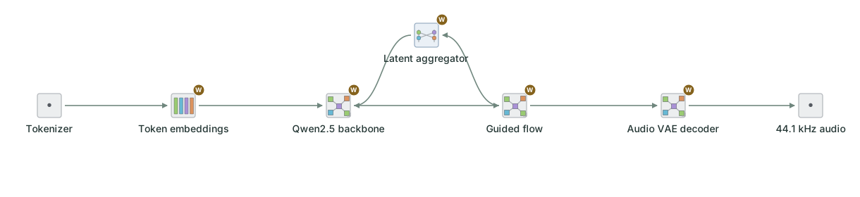
Read the shapes on the wires
Start with one arrow: 1 × 64 leaving Guided flow is one finished patch with 64 coordinates. Follow it up and the aggregator turns it into 1 × 896 for the next backbone step. Follow it right and the decoder waits for a sequence of F × 64, where F counts finished latent frames. Earlier in the diagram, T counts text tokens. Those two lengths measure different things.
A gold W means the stage uses learned parameters. A grey ƒ means its output is computed entirely from its inputs. Think of two matrix products inside attention: XW reads a learned projection, while QKᵀ multiplies two activations. Both can use GEMM. Softmax then turns the scores into attention weights. Those weights change with the sentence; they are computed values, not stored model parameters.
What is Ming’s frontend?
Give the checked CKE runner the sentence “Hello. This is Ming speech.” The first thing it builds is a text prompt. The publisher’s prompt code combines the sentence with the English language setting, the built-in UK_George voice choice and the task instructions. Those choices affect what the backbone sees before it generates a single sound.
Text frontend: sentence + language + voice → formatted prompt → checkpoint tokenizer → ordered token IDs. The runner checks the hash of tokenizer.json before encoding. The IDs are integer addresses. At the next boundary, the embedding kernel gathers a learned 896-value row for each address. Two occurrences of the same ID retrieve the same row. Their positions and neighbors give them different contextual representations inside the backbone. Read the prompt builder and tokenizer adapter.
Where would a microphone recording enter? Whisper starts with samples from a recording and computes log-Mel features for its encoder. Ming can start with typed text and a built-in voice. With a reference clip, the publisher’s audio VAE encoder extracts acoustic latents over time. Its CAM++ speaker encoder can also summarize the voice into a speaker embedding. Both sit on the reference-audio input branch. Publisher’s reference-audio implementation. The pinned CKE runner exercises the built-in voice and rejects reference-audio inputs, so the diagram follows the path we can trace today. CKE’s voice-conditioning scope.
Two loops, two different jobs
The outer loop answers “what comes next in the utterance?” It starts from a formatted prompt, including the chosen voice. The backbone reads that context and the generated runtime checks the stop decision and frame budget. When generation continues, the flow head builds a latent patch. A latent is a compact numerical description of sound. The aggregator converts the patch into a single embedding that the backbone can consume on its next step. Caching the backbone’s earlier keys and values saves it from processing the whole prefix again.
The inner loop answers “how do I turn this noisy patch into one that fits the context?” The diffusion transformer (DiT) predicts a direction of travel. It runs a conditioned branch and a null-conditioning branch. Their difference tells the sampler how much the conditioning changes the prediction. The eight DiT blocks and the sampler steps count different things: one is network depth, the other is repeated refinement.
Follow one patch through the generated circuits
Read the prompt once
The default backbone has 24 layers and a hidden width of 896. An embedding lookup selects one row for each prompt ID. RMS normalization sets its scale before the query, key and value projections. Fourteen query heads share two key/value heads, so each query head has 64 features. Rotary encoding gives the queries and keys their positions. After attention mixes values, a gated MLP expands each row to 4,864 features and projects it back to 896. Residual additions carry the original stream through both sublayers. Read the circuit builder.

Reuse the prefix
At the next position the earlier keys and values are still useful. The cached path seeds them during prefill, then appends the new key and value before mixing values for the new query. This matters when a short sentence has a long voice prompt. The final hidden row supplies conditioning; a separate projection emits two stop logits. The runtime also checks the minimum length and frame budget. Read the circuit builder.

Predict a direction in sound space
The DiT builder takes a 64-wide latent, a conditioning vector of width 896 and the sampler time. It projects them into a 1,024-wide representation. Sinusoidal features tell the predictor where it is in the refinement schedule. Eight transformer blocks with 16 attention heads mix the available positions, and the final projection returns a latent-space prediction. Full attention here can consult the supplied sequence; the autoregressive backbone restricts each query to its permitted context. Read the circuit builder.
Feed one patch back
The aggregator joins a learned class row to the projected patch features. Its transformer stack lets that row collect information from the patch. CKE then selects the class row and returns 896 values: one embedding the backbone can consume next. The original patch takes a second path to the waveform decoder. This fork accounts for the two arrows leaving Guided flow. Read the circuit builder.
Decode only the valid samples
Factor-four interpolation creates four output frame positions per input frame. At an interior position it blends two neighboring frames with weights that sum to one. The 24 decoder layers process the denser sequence, then a spectral head predicts the quantities needed to reconstruct the waveform. The decoder returns a valid sample count. Allocating an arena for a long utterance does not make every sample in that arena part of a shorter utterance. Read the circuit builder.
What exactly goes back to the backbone?
For one 64-value patch, the aggregator projects the patch to 1,024 features and prepends a learned summary row. The resulting matrix has just two rows. Eight attention blocks let the summary row read the patch. After normalization and a learned projection, each row has 896 features. The runtime copies the first row back to the backbone. That one row is the feedback signal for the next patch. Aggregator circuit.
One flow step you can do by hand
Take one coordinate of the latent and call it x. Let p be the conditioned prediction and q the null prediction. Ming’s update uses v = p + cfg × (p − q), followed by x_next = x + dt × v + noise_amplitude × noise. The timestep controls how far to move. The last term is the supplied noise contribution for this step.
For a small example, take x = 0.50, p = 0.30, q = 0.10, cfg = 2 and dt = 0.10. With zero noise amplitude, the guided velocity is 0.70 and the new coordinate is 0.57. Turn guidance down to zero and the same coordinate ends up at 0.53. In CKE, the compiler expresses the vector version with eight scale and sum calls. A swapped input can leave the output shape perfectly valid while changing every subsequent patch.

When does it become a waveform?
The audio VAE decoder reads the finished latents, projects them, upsamples along time and passes them through 24 decoder layers. A spectral projection supplies the information needed to reconstruct overlapping waveform frames. The final stage combines those frames with the specified window and overlap normalization. This path produces 44,100 samples per second.
Take three finished latent frames. The decoder receives 3 × 64, projects to 3 × 896, then interpolates to 12 × 896. Its 24 layers keep that shape. The spectral head predicts 3,530 values per row, two for each of 1,765 frequency bins. Inverse STFT and overlap-add with an 882-sample hop turn those twelve frames into 10,584 samples after cropping. At 44.1 kHz that’s 240 ms of sound. Waveform decoder circuit.

Try the window and hop yourself
A window gives each sample in a short frame a weight. The hop says how far along the signal to start the next frame. In Ming’s decoder those frames overlap on the way back to sound. Start with Overlap-add below. Move the hop from 16 to 64 samples: watch what happens to the overlap envelope when adjacent Hann windows no longer cover each other’s endpoints.
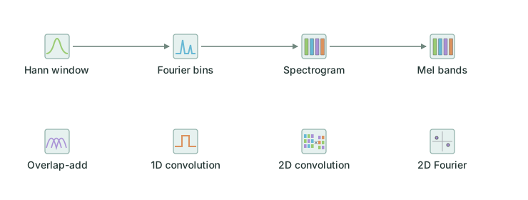
For the analysis direction, select Short-time Fourier transform. The toy signal switches tones halfway through. Increasing the frame length puts the frequency bins closer together, but each column now covers a longer interval. Reducing the hop adds more columns. Follow the same idea in the Whisper frontend. The convolution and 2D Fourier tiles are independent experiments for signals and images.
There’s a useful debugging lesson in the window itself. In a retained comparison, CKE and the publisher received identical spectra but still produced different samples. The publisher rounded intermediate window-normalization values to BF16, and the order in which overlapping contributions were added mattered. Reproducing that behavior brought the reported maximum absolute waveform difference down to 8.94 × 10⁻⁸ for the reference clip. That number measures the reconstruction stage on supplied spectra. Earlier latent differences still have their own path into the final audio.
Ming3, Qwen3-TTS and Kokoro: what goes into the waveform decoder?
Give all three the same sentence. Stop each model just before it produces audio and inspect the data at that boundary. It’s a useful way to see why three text-to-speech systems need different kernels.

Ming3 refines a continuous patch
The text frontend supplies token IDs. The backbone supplies context. The DiT and sampler then make several numerical updates to one patch. Once the patch is ready, the aggregator summarizes it for the next backbone position. The audio VAE receives the sequence of patches. If an update drifts, you can compare the same latent coordinate before and after a single sampler step.
Qwen3-TTS predicts discrete speech codes
In the 12 Hz family, text tokens condition the talker. For an audio frame, the talker predicts the first codebook index and the code predictor supplies the remaining indices. A codebook index selects a learned entry. The codec decoder uses the completed frames to reconstruct audio. Here 12 Hz describes the rate of code frames; each frame expands into many waveform samples. A useful debugging boundary is the complete set of indices for one frame: did the predictions diverge, or did the decoder turn identical codes into different samples? Voice inputs depend on the variant; Base supports reference-audio cloning, while CustomVoice provides built-in speakers. Qwen3-TTS model and voice modes · Explore the Qwen3-TTS circuit.
Kokoro makes phoneme timing explicit
Kokoro’s language frontend converts written text into phonemes, the sound units the model will pronounce. The model encodes those units and predicts how long each should last. Duration expansion repeats their features across acoustic frames. Pitch and noise predictions, aligned text features and voice style then condition the waveform generator. If a syllable sounds rushed, inspect its phoneme sequence and duration first: an incorrect duration changes how many frames the generator gets for that sound. Kokoro language frontend · Kokoro model path · Explore the Kokoro circuit.
These are architecture comparisons. The timing figures later in this article belong to Ming3’s retained CKE runs. A speed or voice-quality comparison would need the same text, hardware and listening protocol across all three.
What ran, and what it tells us
I checked the flow-step and sentence-segmentation tests on CKE revision e61edf9a3. All five passed locally. One compiles the native step and checks its output against each point in a retained five-update FP32 trajectory. Another deliberately changes a graph connection and confirms the reference comparison catches it. The segmentation check makes sure splitting a paragraph preserves its text exactly. These are small tests you can rerun without the full voice checkpoint.
python3 -m unittest tests.test_v8_ming3_flow_step tests.test_v8_ming3_text_segments -vThe full synthesis numbers below come from CKE’s retained development trials. I didn’t rerun those audio jobs for this article.
| Trial | Audio produced | What to notice |
|---|---|---|
| Short prompt, same 32 latent frames | 2.56 seconds | Generation took 552.3 seconds with full-prefix execution and 91.1 seconds with the cached candidate. Waveform decoding took another 14 seconds in each run. |
| 100 words, seven sentence chunks | 48.24 seconds | Generation took 1,583.7 seconds and decoding took 263.4 seconds, excluding load. The result demonstrates completion; it also makes the latency gap easy to see. |
The short trial suggests a practical place to measure next: caching helped the outer loop, but generation still dominated the elapsed time. The paragraph trial raises a different question. Whisper recovered the sentences with one normalized word different. A transcript can miss a clipped consonant, an awkward pause or a rough sentence join. Listening tests, publisher BF16 and random-number parity, and a serving interface are still open.
The 28 kernel bindings behind the circuits
This inventory follows six builders at the pinned revision: full and cached backbone, DiT, aggregator, sampler update and runtime decoder. A kernel appears once even when dozens of layers call it. Open its map for the shape contract and its C source for the arithmetic.
Prompt, attention and cache · 11 kernels
audio_text_embedding_token_major_f32Gather an embedding row by integer ID. The aggregator also uses a lookup to retrieve its single learned class row.
rmsnorm_rows_checked_f32Reduce squared feature values across one row. Scale the row by the inverse root mean square, including epsilon, and apply the learned feature weights.
linear_rows_checked_no_bias_f32Dot each input row with each output weight row. This mixes channels into a new representation without an additive offset.
linear_rows_checked_f32Apply a learned matrix and output bias. Swapping projection weights changes whether the output represents a query, a velocity or stop logits.
layout_token_to_head_checked_f32Move from token-major rows to per-head storage so an attention kernel reads the expected sequence and feature strides.
rope_qk_split_bounded_f32Rotate pairs from different feature halves using the position-dependent phase. This makes relative position visible in the query–key dot product.
attention_sliding_head_major_bounded_f32Compute scaled attention scores over the allowed context, normalize them and use the weights to sum values. The circuit supplies the window bound.
Kernel map · transformer_rows_checked.c · attention_kernels.c · softmax_kernels.c
layout_head_to_token_checked_f32Gather results from separate heads into token rows for the output projection. This rearrangement preserves the numerical values.
kv_cache_seed_checked_f32Write prefill keys and values into the cache layout that continuation expects. Subsequent positions can reuse the prompt.
attention_decode_append_checked_f32Append the new key/value position, score the new query against the valid cache and mix values. Bounds checks keep the append within capacity.
silu_mul_rows_checked_f32Apply SiLU to the gate, then multiply with the parallel MLP branch feature by feature. The down projection consumes this gated row.
Patch prediction, guidance and feedback · 11 kernels
sinusoidal_features_f32_checkedEncode the sampler time with multiple sine and cosine frequencies so the DiT can respond differently early and late in the trajectory.
sinusoidal_constant_tables_f32_checkedConstruct sine and cosine coefficient tables from declared frequencies. Later position rotations reuse these tables.
rope_pairwise_rows_f32_checkedRotate adjacent features in pairs using supplied tables. Pair ordering matters: a different pairing can produce plausible shapes and incorrect attention.
attention_full_token_major_f32_checkedCompute attention over the full short sequence. The class row in the aggregator can therefore collect information from the patch positions.
gelu_rows_tanh_checked_f32Apply the tanh approximation of GELU to each feature between two learned projections. This gives the MLP a nonlinear response.
Kernel map · gelu_rows_tanh_checked.c · gelu_kernels.c · ckernel_strict.c · ck_threadpool.c
silu_strided_f32_checkedCompute x times sigmoid(x) at the declared strides, preserving the layout expected by the conditioning projection.
audio_concat_channels_checked_f32Join two logical channel ranges with explicit strides. The following operation sees the assembled representation in its declared order.
scale_vector_checked_f32Multiply a vector by one scalar. The sampler reuses it to apply coefficients to differences, velocities and noise.
audio_scaled_sum_strided_f32_checkedCombine corresponding elements with a supplied scale. Its connections determine whether the result is a residual sum, guided velocity or state update.
audio_noise_counter_gaussian_f32Produce Gaussian samples from a counter-based random stream. Identical seeds in two different generators need not give identical noise.
runtime_copy_valid_f32Copy only the declared valid extent. In the feedback path this hands the selected representation to the next consumer.
Waveform and valid lengths · 6 kernels
audio_upsample_linear_frames_f32_checkedMap each output frame center to a fractional input position and interpolate between its neighbors. Clamp at the ends where a second neighbor is unavailable.
audio_spectrum_cartesian_f32_checkedConvert predicted magnitude and phase into real and imaginary frequency bins with the declared clamps. The inverse transform consumes these bins.
audio_istft_complex_window_f32_checkedInvert each spectrum, apply the stored window, overlap-add the frames and normalize by the window envelope before cropping the ends.
runtime_extent_sum_i32Add runtime lengths under the declared capacity. Downstream calls use the valid rows even when their buffers are larger.
runtime_extent_scale_i32Multiply a valid length by a factor, for example converting a row count into the number of feature elements to process.
runtime_extent_affine_i32Apply a scale plus an offset to a valid length. This expresses the effect of upsampling and endpoint crops on output sample count.
From one flow update to connected speech
5 linked changesMing3 development history
- PR #1129Compile the guided update with shared scale and sum kernels4e0cf6bb1
- PR #1131Add checked half-pixel interpolationa7a627765
- PR #1132Match the BF16 fold during waveform reconstruction75a399437
- PR #1138Connect latent frames to the generated audio decoder550749f27
- PR #1141Connect native generation, feedback and valid decoder lengthse1c9696bb



Comments
Join the conversation. Replies can go three levels deep.